Realtime classification in Pathway

Part 2: The Nearest-Neighbors classifier under the hood: classification using kNN and LSH

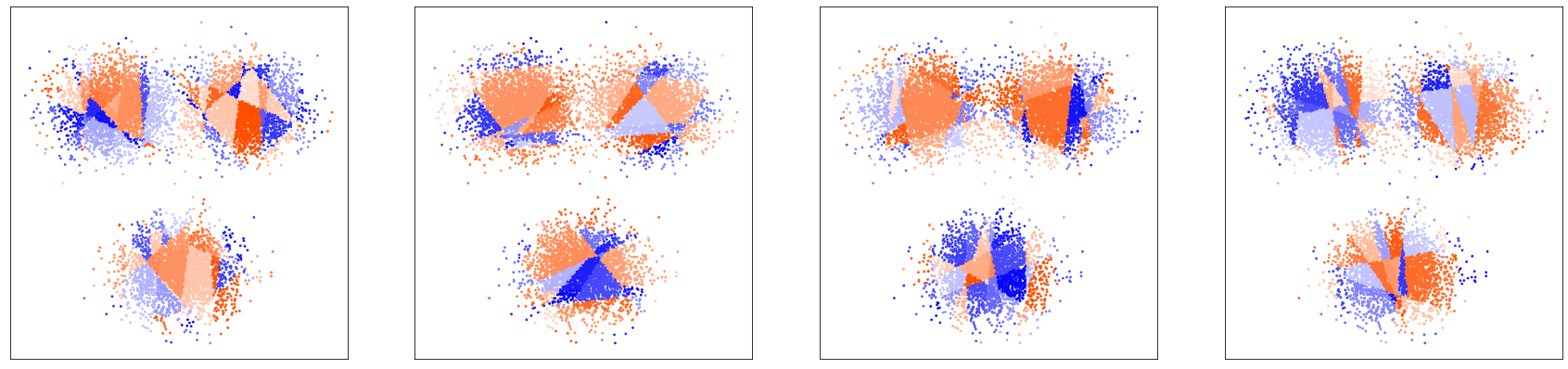
Figure: Dimensional segmentations of space made by four different LSH projections.

Today, we will explain how our classifier works and present to you the two main concepts behind it: kNN and LSH.

In this article, we are not going to explain what classification is and how easy it is to create a classifier with Pathway, as we already have an awesome article about it.

Deep dive: how we wrote the kNN+LSH classifier

kNN explained

The k-Nearest-Neighbors (kNN) classifier relies on the following assumption: if some datapoints have a given label, and your query is similar to those datapoints, then your query is likely to have the same label as them.

The kNN classifier assumes that a pool of already labeled data is available. The kNN approach connects each query to its k closest counterparts in the dataset, called 'neighbors'. In a nutshell, each query is connected to the k other data points of the dataset which are the most similar to it. The assumption is that similar data points are likely to share the same characteristics: the query is likely to share the same label as those of its neighbors.

"Friends are like mirrors. You can see yourself just by looking at them."

For classification, the label is chosen by a majority vote among the labels of neighbors of the query.

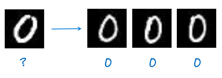
In this example, the image we want to label is connected to its k=3 nearest neighbors. Given that those images are labeled as '0', we can also label the image as a '0' too.

One reason of the success of the kNN approach is its simplicity: its vanilla version can be implemented very easily and is highly accurate. Furthermore, contrary to many of its competitors, the kNN approach is not a black box: the decisions are straightforwardly explainable. Explainability highly increases the trust of users in the system.

The kNN approach is:

• simple
• highly accurate
• explainable

Those are the reasons the kNN approach is widely used for classification or regression, in many fields such as computer vision or item recommendation.

Making sure kNN is fast enough

The 'vanilla' kNN approach relies on a brute force approach to provide the exact k closest data points for each query: a query is compared to all the data points in the dataset. The k closest datapoints, k being a user-defined constant, are returned for each query point.

In Pathway, we are working with large datasets with high-dimensional data. On such datasets, this naive approach suffers from the following issues:

• Time complexity is large:
  • Computing distance between every pair of points is $O(d{n}_t{n}_q)$, where $d$ is the number of dimensions, $n_t,n_q$ number of training, query points, respectively.
  • That can get costly pretty easily. The naive approach is unusable for large data sets.
• Handling updates is expensive/non trivial:
  • When a new batch of data points arrive then distances to all the queries need to be updated. This can be quite a waste of resources.
  • When a batch of data points is deleted or updated then answers to all the queries need to be recomputed.

This vanilla approach is likely to be too slow when a lot of labeled data is available. Fortunately, we can trade quality slightly in exchange for a big speed increase.

The key intuition is to lower the number of potential candidates to be neighbors to limit the number of distance computation. Reducing this pool of candidates speeds up the process: for example, by considering only half the dataset via random sampling, we can reduce the query time by half.

This process comes with a loss in quality: by taking the risk of missing the 'real' neighbors, we take the risk of misclassifying the queries.

The major challenge is then how to select the best candidates to compute the distances from?

To hit a sweet spot, we use a technique called Locality Sensitive Hashing (LSH), to get a kNN+LSH classifier.

Introducing Locality Sensitive Hashing (LSH)

Locality Sensitive Hashing (LSH) is one of the most widely used techniques for speeding up kNN computation. LSH clusters the data into buckets and the distances are only computed between the query and the data points in the same buckets. LSH refers to both hashing functions used for the clustering and the kNN algorithm relying on such functions. LSH functions cluster data points so that the closer the data, the more likely they will be clustered in the same buckets. Such a function highly depends on the targeted distance: the choice of the LSH function is generally imposed by the considered distance. We recommend this great explanation of LSH.

LSH is entirely different from typical hash functions, e.g. for cryptographic purposes, which are designed so that similar objects are hashed to a very dissimilar buckets.

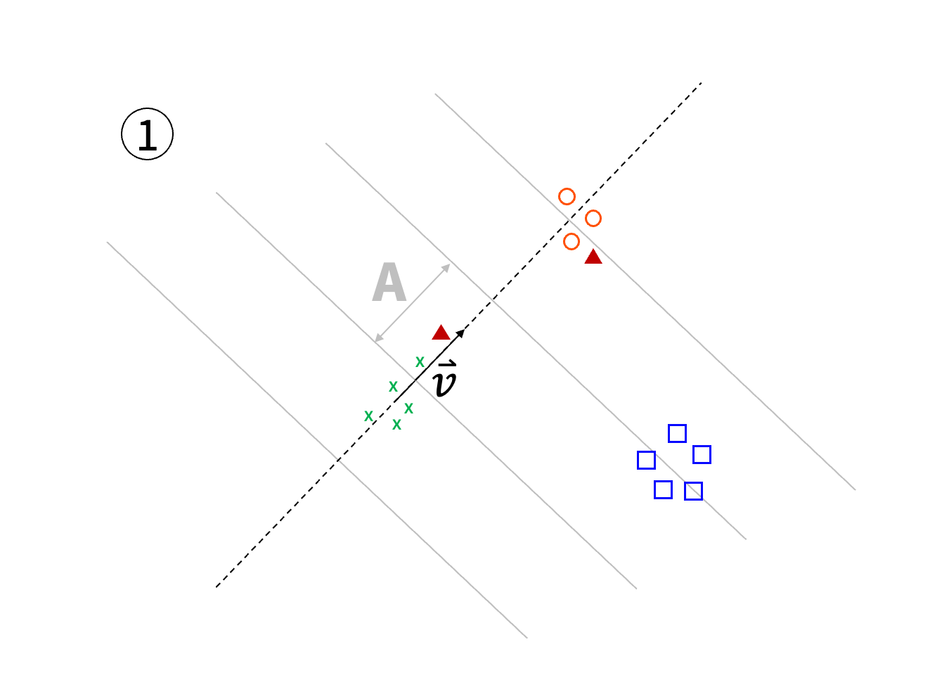
LSH can be described for different distance metrics. When we want to consider Euclidean distance between data points, LSH partitions the space by doing random projections. A random vector $v$ is chosen and a random bias $b$ is used to offset the vector. All the data points are projected onto the resulting line and are assigned in contiguous buckets of width $A$.

In a more formal way, each data point $p$ is assigned by the function $h_{v,b,w}$ to its 'bucket' $h_{v,b,w}(p)$: $h_{v,b,w}(p)=\lfloor \frac{p.v+b}{A}\rfloor$

However, the resulting clustering can be quite coarse. In order to limit the size of the clusters, those are split again by using the same process $M$ times: for two data points to be in the same bucket, they shall have been projected $M$ in the same 'sub-bucket'.

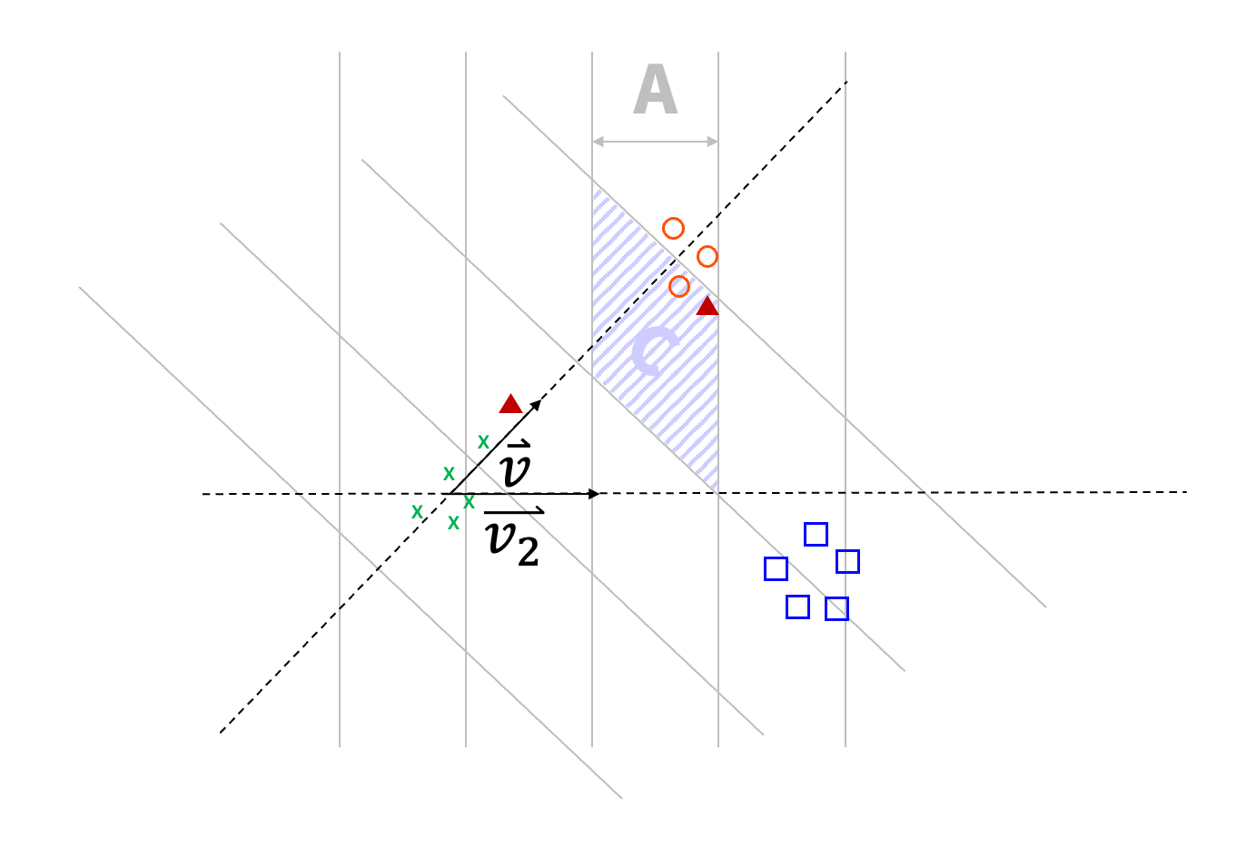
This whole process is repeated $L$ times in order to increase the probability that two close data points are into the same bucket at least once.

LSH clustering scheme:

1. Consider a line using a random vector and partition this line in buckets of width $A$.
2. Project all the points on the line, and put the points in the associated buckets.
3. Repeat steps 1-2 $M$ times and merge the intersecting buckets.
4. Repeat steps 1-2-3 $L$ times.

The LSH index is now ready for computing kNN queries!

The kNN of a query $q$ is obtained by gathering all the data points which are in the same buckets as $q$. Then a standard kNN algorithm on this subset of data points is performed.

LSH query scheme:

1. Find the buckets associated to the query
2. Compute the distance between the query and all the points in those buckets
3. Return the k closest data points

kNN+LSH classifier, Pathway style:

Depending on your classification problem, you may need different distance metrics and thus different projection schemes.

Don't worry, Pathway has you covered, and already provides several such classifiers.

Here is an example of the results Pathway provides:

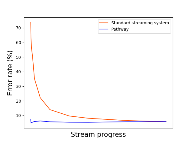
If you haven't done it yet, you can read this article to know how we got this graph, and why Pathway outperforms standard streaming systems.

Conclusion

You now have a good insight on how to do a classifier using kNN queries and how to use LSH to make it scalable.

Pathway already provides ready-to-use classifiers, but the best classifier is one made specifically for your problem: you can easily create your own classifier using Pathway, this is exactly what Pathway is made for!