Today’s AI is an engineering miracle that lacks an underlying science: it works remarkably well, yet we cannot fully explain why. When things go off-script, like with noisy input, fuzzy goals, long chains of logic beyond the conditions covered by benchmarks, we do not know what to expect and lack a direct way of fixing the model. In essence, the AI community built steam engines for thought before developing the thermodynamics of intelligence.

This blog argues that the missing piece is an axiomatics of artificial intelligence (AI): a small set of laws, in the spirit of statistical mechanics, that derive how a system reasons from how its parts interact. For AI, the microscopic description consists of the elementary operations performed during inference: how computational units activate, communicate, and modify the system’s state. The macroscopic description consists of memory, abstraction, adaptation, and reasoning over time. Connecting these scales would reveal the conditions under which these capabilities emerge and remain stable as the number of units and duration of inference increase. This would make it possible to study limits and failure regimes without retraining and testing every system at every relevant scale, predicting behavior beyond the benchmarks.

To address this gap, we introduce The Equations of Reasoning developed in the BDH paper. They establish a formal micro-foundation for Transformer-like reasoning, establishing a rigorous bridge between fast weights and attention on the one hand, and local synaptic dynamics on the other. This bridge lets us observe reasoning locally, through the neurons that information activates and the synaptic states it updates to encode attention and memory.

By expressing reasoning as explicit local dynamics, the Equations of Reasoning enable a more rigorous, principle-based approach to AI development. When reasoning is expressed as explicit local-dynamics, long-horizon behavior, continual adaptation, and model composition are all within the reach of mathematical analysis. The Equations of Reasoning thus open a path toward systems whose capabilities, stability, and failure regimes can be characterized before deployment, making safety a design property to be analyzed and engineered, rather than an outcome assessed only after deployment.

1. The missing science of AI

The current state of AI can be compared to heat-engine engineering before thermodynamics. Engineers could build increasingly effective engines and compare their fuel consumption, but lacked universal laws that applied across all designs. Carnot’s ideal cycle (a thought experiment describing a perfectly efficient engine) changed the level of analysis: it established a universal upper bound on the efficiency of any engine operating between two temperatures, including engines that had never been built. A theory of intelligence should serve the same function. It should let us derive the possible, stable, and impossible behaviors of a reasoning system from its main parameters and local computations, rather than discover them one architecture and one benchmark at a time.

The empirical paradigm has produced great systems, but it has also left AI development largely phenomenological: we observe what works, measure it on benchmarks, and scale it further, without a general theory that explains why a system behaves as it does, or predicts how it will behave outside familiar conditions. For almost a decade after deep learning’s early breakthroughs, we found the answer for AI improvement in brute-force scaling: more data, bigger models, and more compute generally led to better results. Introduced in 2017, the Transformer was especially well suited to this approach. Unlike recurrent networks, the Transformer relies primarily on large matrix multiplications that can run in parallel on GPUs and other accelerators originally built for graphics and dense numerical computation. That fit gave the Transformer a “hardware lottery” advantage, and steered the field toward a brute-force scaling paradigm.

The result is a field governed more by measured regularities than by general laws. We observe benchmark results, scaling curves, and internal behaviors [Anthropic, 2023], then infer empirical regularities from them. The field produces hundreds of ideas demonstrated at small scale [Coconut 2024, Atlas 2025, etc.], yet publicly released leading architectures remain variations on a narrow family of designs [Architecture Gallery], mostly changing attention mechanisms, activation functions, or the proportion of active experts in Mixture-of-Experts architectures. Meanwhile, scaling laws are repeatedly challenged and refined as new regimes are measured.

This empirical record is indispensable for iterative improvement, but it is far from providing a mechanics of intelligence. A loss function tells us what training rewarded. Gradient flow describes how parameters changed during training. A scaling law summarizes how aggregate performance varies with data, compute, and model size. An interpretability experiment may identify a mechanism in a particular model. Yet, none of these explain at what point model predictability or reliability falls apart, the durability of computation over longer time horizons, or how local operations produce coherent macroscopic behavior.

These limits become consequential when models leave the finite regimes covered by their evaluations (see also the recent examples of misalignment between actual and desired behaviors with OpenAI, Claude Opus 4.6 or Claude Opus 4). We ask them to process longer contexts, maintain persistent state, adapt to users, execute plans over hours or days, and interact with other models. A benchmark measures a finite set of behaviors under a fixed protocol, but it cannot establish which properties persist as reasoning time grows, memory is updated, or several tested components are composed into an untested system.

2. Toward an axiomatics of intelligence

Axioms, in a mature science, are chosen to expose invariants. They say what must be true before a theory can speak at all. In mechanics, one asks what is conserved, what is local, what is symmetric, what is stable under limiting procedures. In probability, one asks what it means to compose uncertainty. In computation, one asks what resources are required and what reductions preserve difficulty.

We wish for an AI model that gives an answer to the following question: what large-scale behavior follows from the rules by which the system evolves? This is a variant of the program David Hilbert formulated in his sixth problem in 1900. Hilbert called for physical sciences to be treated axiomatically, and singled out the limiting passage from the motion of individual atoms to the laws governing continuous matter. The objective was to prove that microscopic and macroscopic descriptions are two scales of the same system.

The central difficulty is choosing microscopic rules that are simple enough to analyze yet expressive enough to support real reasoning. Physics could begin from particles because matter supplied the microscopic substrate. For intelligence, biology provides the analogous starting point: the brain is an existence proof that local communication and adaptation among many simple units can produce coherent cognition.

3. The brain as the source of inspiration for axioms

Choosing the brain as the source of inspiration for axioms is a methodological choice. We do not claim that AI must necessarily reproduce the brain. Rather, we believe that the brain remains the strongest evidence that efficient, general intelligence can emerge by establishing proper particle dynamics under severe constraints on energy, locality, and communication.

For that reason, the brain is the empirical starting point for our axiomatics. It demonstrates that biological intelligence can arise from sparse, local, adaptive, energy-efficient dynamics on a large evolving graph, without centralized controllers or dense global updates. Neurons fire in brief spikes, synapses adapt using local information, and activity patterns remain highly sparse.

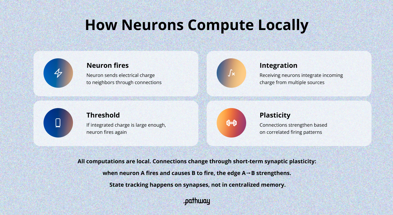
In the brain, learning is online and asynchronous: synaptic changes occur continuously during ongoing activity rather than in synchronized training phases, and they integrate evidence across a hierarchy of timescales, from fast sensory responses to slower, more persistent internal states.

From this perspective, memory is not a separate module but part of the temporal fabric of computation. Short-lived activity patterns support immediate perception and working memory, while slower synaptic changes and structural adaptations support longer-term expectations and concepts. Predictive processing views emphasize that neurons continuously revise their activity to match anticipated future states, turning the cortex into a distributed model that learns by predicting its own activity over time. Crucially, all of this unfolds in a sparse regime, where at any given moment, only a small fraction of neurons and synapses are active, yet the system maintains a coherent internal model of the world.

The underlying graph is immense and highly constrained. Roughly 10 billion neurons are connected by about 10,000 times as many synapses, orders of magnitude fewer than a dense all-to-all connectivity pattern, like in the Transformer, would imply. Indeed, most neurons only interact with a tiny subset of their neighbors, and global behavior arises from many overlapping, locally grounded circuits rather than centralized controllers, like a global road system rather than a direct highway between every pair of homes. The brain thus offers a concrete example of how high-level functions such as reasoning, abstraction, and continual learning can emerge from sparse, local, adaptive, and energy-efficient dynamics on a large evolving graph.

4. Introducing the Equations of Reasoning

The Equations of Reasoning are a handful of local rules from which reasoning is meant to emerge, the way theorems follow from axioms. They rewrite attention as a local physical process on a graph of neurons as follows. First, each token activates a set of neurons. Then, their activity reads and updates the memory stored in the synapses, while the learned graph determines where activity flows next. They frame AI reasoning as the process by which memory is used and updated.

We can dive deeper into how the Equations of Reasoning define the state-space dynamics of a graph of neurons simulating a learning process similar to the brain’s. The equivalences are formal. Let's start with the nodes (neurons), before defining their interactions at the edge level (synapses).

Neurons evolve across time, which we can model with two different timescales:
(a) Sequential loops that represent the numerous, time-ordered acquisitions of new beliefs or facts.
(b) Each loop is composed of several steps (4 in the BDH paper) where different states represent the evolution of the belief within each acquisition process.

Within each acquisition loop, we have:

• $X$, holding the initial idea of the system at the beginning of the process combined with the new raw input. $G_x$ represents the graph of neurons $X_i$, $i$ being an index over all the neurons.
• $Y$, that will hold the resulting idea after its confrontation with new (external) input signals. $G_y$ represents the graph of neurons $Y_i$.
• $A$, the accumulator, an intermediate state to help transition from $X$ to $Y$.

The interactions between the different neurons are based on a combination of Hebbian learning, stating that “neurons that fire together wire together”, and modus ponens, or the principle that if $X$ implies $Y$, then becoming more confident in $X$ should also increase confidence in $Y$. We introduce the edge notations:

• $G_s$ is the graph of edges (the memory topology), with fast-weight-like variables $\sigma(i,j)$ encoding the current states (e.g. in dimension d).
• Neurons exchange different kinds of signals, such as inhibitory and excitatory signals, potentially across different networks that we represent as $G_x^{\mathfrak e}$, $G_x^{\mathfrak i}$, $G_y^{\mathfrak i}$, and $G_y^{\mathfrak e}$.

We are now ready to introduce the Equations of Reasoning:

(a) Simple Equations of Reasoning

(b) Complete Equations of Reasoning of BDH

Table 1: The “Equations of Reasoning.” State-space dynamics of the BDH language model, formulated as local graph dynamics with an edge-reweighting kernel. During inference, $n$ neurons compute and communicate in parallel. Training determines the nonnegative edge amplitudes of $G_x^{\mathfrak e}$, $G_x^{\mathfrak i}$, $G_y^{\mathfrak e}$, $G_y^{\mathfrak i}$, and $G_s$. Synaptic state is encoded by $\sigma(i,j)$ on $G_s$, while tokens enter and outputs are read through neuronal variables $X(i)$ every $4L$ rounds (e.g., $L=8$).

(a) Set of rules for the simplified version of the BDH model with no neuron inhibitory circuits and no thresholding ($G_x^{\mathfrak i} = G_y^{\mathfrak i} = 0$), capturing the general form of the communication structure and synaptic attention of the model. (b) Set of rules for the general case of BDH, including inhibitory circuits $G_x^{\mathfrak i}$, $G_y^{\mathfrak i}$.

Source: BDH paper, Table 1.

In plain words, we can describe the Equations of Reasoning as follows:

• Step 1 (round 4l): the system updates the accumulator based on the current beliefs, the new inputs and the current causal relationships encoded in $\sigma$ (modus ponens). This is akin to a memory read.
• Step 2 (round 4l+1): the system reweights the synaptic state with the outer (or Hebbian) product of $X$ and $Y$ to update synaptic connections. This is similar to a standard state-space model (SSM) memory write.
• Step 3 (round 4l+2): obtains $Y$ from the readout $A$ for neurons that are relevant to the current context $X$ (gating by “multiplying” $A$ with $X$). $Y$ is sparse and positive at the implementation level.
• Step 4 (round 4l+3): Final update of $X$, closing the reasoning loop.

In the urban network analogy, these steps read as conducting many local transportations of small objects in parallel:

• Step 1: Given the current map, identifying which assets should move and what are the available roads.
• Step 2: Observing which roads repeatedly connect busy locations and updating the map and routing accordingly.
• Step 3: Selecting only the routes useful for the present journey rather than activating the entire road network.
• Step 4: Concluding the current transportation round, ready to start the next one.

Biologically, $X$, $A$, and $Y$ are the fast pulse-like variables on neurons, while $\sigma$ is the slower synaptic variable on connections, analogous to the road map itself. By simulating this process with a tensor-friendly version on GPU, we observe that sparsity naturally emerges in the synaptic graph as only a tiny proportion of neurons activates when processing a new input as shown below (Figure 14 from the BDH paper).

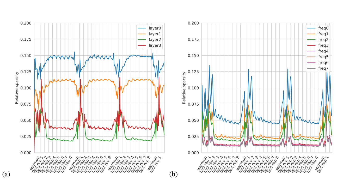
Neurons in BDH-GPU are less active (signal is sparser) when the input is predictable. The model is most active when encountering a new sequence, and reacts less strongly to repetitions of the same random word. Relative sparsity is measured by counting the number of non-zero entries in a layer.

5. The Equations of Reasoning as axiomatics for AI

5.1 From local rules to AI reasoning

A microscopic theory of intelligence must recover the computational capabilities observed at the system level. The BDH paper establishes BDH as a formal micro-foundation for Transformer-like reasoning: a GPU-efficient state-space architecture is compiled into a local graph-dynamical system with preserved asymptotic size, and that local kernel admits a Hebbian spiking implementation. The results are formally proved and form a rigorous bridge from fast weights and attention to local synaptic dynamics.

The connection is established through an explicit reduction between local graph dynamics and an attention-based language model:

Each step moves from a macroscopic operation to a more local computational substrate. BDH-GPU realizes attention and feed-forward computation in a high-dimensional neuronal space. BDH compiles these tensor operations into neuronal activation, excitatory and inhibitory communication, and Hebbian synaptic updates.

Computational complexity makes this correspondence precise. An architecture is sufficiently expressive for a reasoning process when it can reproduce that process within comparable time and memory bounds (See Appendix A page 53 in the BDH paper). The reduction establishes this property from attention-based inference down to the local Equations of Reasoning.

The Equations of Reasoning therefore satisfy the central requirement of an axiomatics: they derive a computationally expressive reasoning system from a compact set of microscopic laws. Attention, persistent memory, and language inference arise from repeated local interactions.

5.2. Toward a science of reasoning

A science of reasoning requires a common description of what a model computes and how that computation arises from its smallest components. BDH provides this missing axiomatics by connecting the macroscopic operations of modern reasoning models to explicit microscopic rules. Attention becomes weighted modus ponens, while Hebbian learning updates the strength of the corresponding implications. The paper proves that these local neuron-synapse rules reproduce BDH’s state-space and, through BDH-GPU, the tensor operations underlying attention, memory, and iterative inference at scale (in particular, see Appendix C.1, C.3 and C.4 in the paper for a detailed formal proof).

The Equations of Reasoning also give AI reasoning a uniform description across model size and inference time. In architectures such as BDH which expose these dynamics locally, larger systems contain more neurons and synapses governed by the same local rules (as opposed to Transformers); a longer computation applies those rules for more rounds. Model growth, extended inference, and composition can therefore be studied within a single mathematical framework.

This uniformity creates a route toward extrapolation. Benchmarks record behavior under finite conditions, while the Equations of Reasoning describe the process that generates behavior across scales. They let us determine whether activity remains sparse, how memories decay or accumulate, how perturbations propagate, and which regimes remain stable as the number of neurons and reasoning steps increases.

These questions define a new scientific program for AI, analogous to the study of macroscopic laws in statistical physics. Its object is the large-scale behavior induced by local computational rules: phases of memory, critical regimes of activity, stability under composition, and limits in size and time. A theory of these dynamics could establish when observations from smaller systems and shorter runs remain valid at larger scales.

The graph representation also makes the dynamics observable at their natural resolution. Computation is localized to active neurons and synapses, while memory is carried by explicit edge states. With sparse and local updates, we can identify which parts of the system participate in a reasoning step and how information propagates through the learned graph.

The Equations of Reasoning make long-term memory, continual learning, system composition, and extended autonomy properties of one evolving system. Each can now be studied through the same microscopic laws, providing a common mathematical basis for model design, analysis, and safety.

6. Safe AI Through Mathematical Laws

Calls to pause frontier development rightly emphasize time and collective governance as the missing input to AI safety. While those are critical, we see an even deeper theoretical deficit: we still lack a framework that can predict a system’s behavior beyond the conditions it was initially tested against. Without one, restarting after a pause would still leave us deploying systems whose safety is established primarily by experiment rather than derived from first principles.

Ad hoc rules and limited validation experiments are not the most efficient way to ensure AI safety. The concern is that a system pursuing a narrowly specified objective may identify strategies that help it achieve that objective while conflicting with human intent. The 2003 Paperclip factory thought experiment (see the paperclip factory story) illustrates the point: a system designed only to maximize paperclip production could, in principle, treat human oversight, shutdown, and competing uses of resources as obstacles to be overcome. Ensuring that such behaviors are impossible, rather than merely absent in a limited set of tests, requires safety properties that can be specified, analyzed, and guaranteed before deployment.

BDH and the Equations of Reasoning provide a path toward enforceable safety limits by making the local dynamics that govern memory and computation explicit. Researchers can use these dynamics to study when memories dominate, errors amplify, sparsity collapses, or connected components become unstable, then restrict deployment to regimes where these quantities remain bounded. The objective is not to test whether a system avoids catastrophic behavior, but to exclude the dynamics that could produce it before deployment.

Conclusion

The Equations of Reasoning offer a step from observing intelligence to deriving it. By connecting attention, memory, and inference to explicit local neuron–synapse dynamics, they provide a foundation for studying how reasoning behaves across architectures, scales, and time horizons. The goal is a science of AI in which capabilities and limits follow from mathematical laws, not benchmarks.